Introduction to Linear Programming
I’ve always been fascinated by making things work efficiently, especially in designing control systems. One area that I want to talk about to day is Linear Programming (LP), which is a key aspect of optimization theory. Optimization techniques are widely used in control systems such as Linear Quadratic Regulator (LQR) and Model Predictive Control (MPC).
What is Linear Programming?
Linear Programming involves optimizing (either minimizing or maximizing) a linear objective function subject to linear equality and inequality constraints. The formulation of a typical LP problem looks like this
\[\\ \begin{align} \min_{x} \quad & {\bf f}^T {\bf x} \tag{1.1}\\ \text{s.t.} \quad & {\bf Ax} \leq {\bf b} \tag{1.2}\\ & {\bf A}_{eq} {\bf x} = {\bf b}_{eq} \tag{1.3}\\ & {\bf l}_{b} \leq {\bf x} \leq {\bf u}_{b} \tag{1.4} \end{align} \\\]where
- \({\bf f}^T\) is the transposed vector of coefficients.
- \(\bf x\) is a vector of optimization variables.
- \(\min\) stands for minimize
- s.t. stands for “such that” (and “subject to”).
- The lower part under s.t. defines the equality and inequality constraints.
- \({\bf A}\) and \({\bf A}_{eq}\) are matrices for inequality and equality constraints, respectively.
- \(\bf b\) and \({\bf b}_{eq}\) are vectors for inequality and equality bounds.
- \({\bf l}_b\) and \({\bf u}_{b}\) represent the lower and upper bounds of the variables.
The goal is to minimize the linear objective function \({\bf f}^T {\bf x}\). Maximizing the the objective function is equivalent to minimizing its negative.
Example Problem: Solving LP in MATLAB
Let’s look at a simple example of solving a Linear Programming problem using MATLAB. Given the following vectors:
\[{\bf f} = \begin{bmatrix} 2 \\ -4 \\ 10 \end{bmatrix}, \quad {\bf x} = \begin{bmatrix} x_1 \\ x_2 \\ x_3 \end{bmatrix} \tag{1.5}\]We aim to minimize \({\bf f}^T {\bf x}\) subject to given constraints:
\[\\ \begin{align} \min_{x_1,x_2,x_3} \quad & 2x_1 - 4x_2 + 10x_3 \tag{1.6}\\ \text{s.t.} \quad & 6x_1 + 3x_2 + 2x_3 \leq 140 \tag{1.7}\\ & 3x_1 - 3x_2 + 4x_3 \leq 60 \tag{1.8}\\ & x_1 + 3x_2 + 12x_3 = 20 \tag{1.9}\\ & 3x_1 + 2x_2 + 3x_3 = -10 \tag{1.10}\\ & -1200 \leq x_1 \leq 1200 \tag{1.11}\\ & -900 \leq x_2 \leq 900 \tag{1.12}\\ & -1300 \leq x_3 \leq 1300 \tag{1.13} \end{align} \\\]This constraints of this problem can be expressed in matrix form:
\[\\ \begin{align} {\bf Ax} \leq {\bf b} \tag{1.14}\\ {\bf A}_{eq}{\bf x} = {\bf b}_{eq} \tag{1.15}\\ {\bf l}_b \leq {\bf x} \leq {\bf u}_b \tag{1.16} \end{align} \\\]The MATLAB code for solving this problem using the “linprog()” function is:
f = [2 -4 10];

A = [6  3  2 ; 3 -3  4];
b = [140 ; 60];
Aeq = [1 3 12 ; 3 2 3];
beq = [20 ; -10];
lb = [-1200 ; -900 ; -1300];
ub = [1200 ; 900 ; 1300];

options = optimoptions('linprog','Algorithm','interior-point','Display','iter',...
          'MaxIterations',1500,'OptimalityTolerance',1e-9,'ConstraintTolerance',1e-6);

[x,fval,exitflag,output] = linprog(f,A,b,Aeq,beq,lb,ub,options)
In this code:
- “linprog” is the function that solves LP problems.
- The “interior-point” algorithm is chosen, but other algorithms can be used as well.
- We set the maximum number of iterations (“MaxIterations”) to 1500.
- “OptimalityTolerance” and “ConstraintTolerance” are set to ensure precision.
Solution Analysis
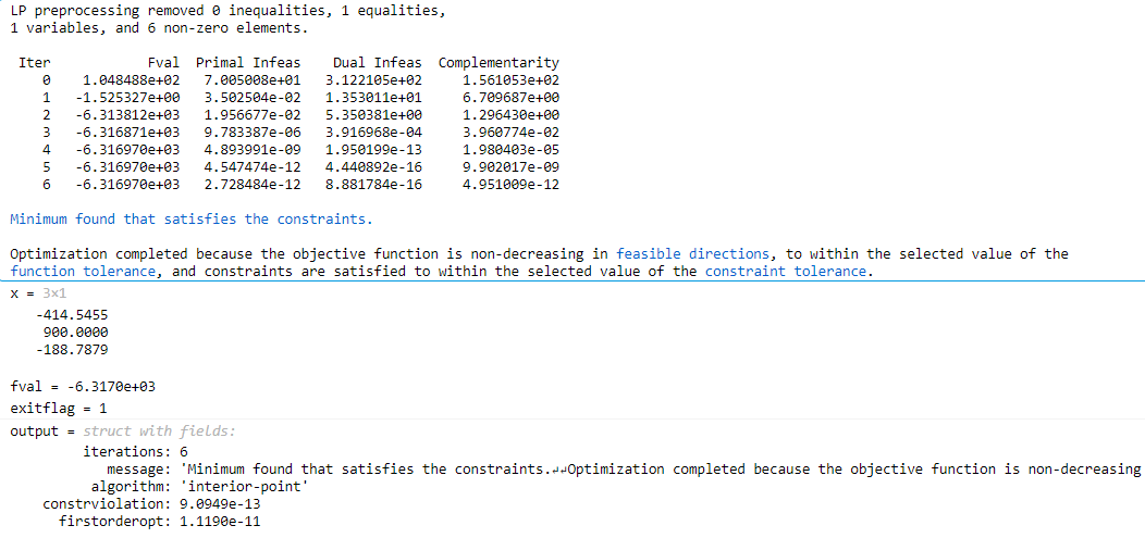
After running the MATLAB code, the output will provide the solution to the optimization problem:
- \(x\) gives the optimal values of the variables.
- “fval” is the minimized value of the objective function.
- “exitflag = 1” indicates a successful solution. Any other value suggests issues with the solution process.
- “output” provides more details on the iterations and steps.
For this problem, the optimal solution is:
\[\\ \begin{align} {\bf x} = \begin{bmatrix} x_1 \\ x_2 \\ x_3 \end{bmatrix} = \begin{bmatrix} -414.5455 \\ 900 \\ -188.7879 \end{bmatrix}. \tag{1.17} \end{align} \\\]As we can see, \(x_2 = 900\) exactly meets the upper bound constraint for \(x_2\), limiting the solution.

Figure 1: Solution to the linear programming problem above. The figure shows the output from the linprog() function in MATLAB.
Linear Programming is just the beginning of constraint optimization. A more useful topic in control systems is Quadratic Programming (QP).
Useful links related to Optimization Programming:
References
[1] Linear Programming. Wikipedia. Link to reference
[2] Matlab. Linear Programming. Link to reference
[3] Matlab. Linear Programming Algorithms. Link to reference